Abstract
Cluster thinning is practiced to reduce grapevine crop load and advance ripening parameters, such as soluble solids, which may or may not lead to higher quality wine. It is often implemented in the field with little or no specificity, and its practicality has been questioned because of increased production costs and lost yields. New analytical methods are introduced that combine commonly available yield and cost data with estimated parameters for grape quality and willingness-to-pay. The result is a tailored economic model that allows growers to calculate their optimal yields and prices within a rigorous, quantitative decision-making framework.
Growers of premium winegrapes face a common dilemma between the potentially incompatible demands of simultaneously increasing yield and increasing quality. These two goals may seem irreconcilable because of a historically tenuous belief that lower yields lead to better wine. The Ravaz index, which is the crop-load ratio of fruit weight per unit pruning weight (Ravaz 1911), is one of the most important indicators of vine physiological balance (Smart 1995). Yet, the Ravaz index is primarily useful to the extent that its measurements can be predictably calibrated with fruit and/or wine quality at both low and high boundaries of acceptability—a range between 5 and 10 (Bravdo et al. 1984, 1985). This principle has been subject to dozens of investigations on various cultivars grown in warm and dry (Chapman et al. 2004, Keller et al. 2005) and cool and wet (Reynolds et al. 2007) growing conditions. However, the existence of a crop-load metric to indicate vine balance by itself does not necessarily enhance decision-making acuity among grapegrowers, particularly in regions where prices are not directly based on fruit quality.
The most common method of reducing crop load is through cluster thinning (CT). When a commercial grower thins clusters after yield estimation to intentionally reduce crop load, it is generally done with the basic premise that the lost revenue from lower yields will be recaptured through increased prices resulting from changes desired by the buyer, such as higher soluble solids or increased flavor. Typically, CT is used to advance ripening in red cultivars or in regions with shortened growing seasons (Jackson and Lombard 1993, Keller et al. 2005, Reynolds 1989). However, CT can be used to advance the timing of fruit maturity or increase soluble solids in white cultivars as well, including Riesling in southern Australia (McCarthy 1986) and western Canada (Reynolds 1989, Reynolds et al. 1994), Chardonnay Musqué in eastern Canada (Reynolds et al. 2007), Seyval blanc in the northeastern United States (Edson et al. 1993, 1995, Reynolds et al. 1986), Chasselas in southwestern Switzerland (Murisier and Ziegler 1991), and Trebbiano in northern Italy (Arfelli et al. 1996). Yield components are also affected by CT, and some field studies have shown that the average cluster weight at harvest is higher for thinned vines compared to nonthinned control vines, including Gewürztraminer (Reynolds and Wardle 1989), Riesling (Reynolds 1989, Reynolds et al. 1994), and Seyval blanc (Edson et al. 1993, Kaps and Cahoon 1989, Reynolds et al. 1986).
Since vine yield is generally the major economic consideration of grapegrowing, and there are costs associated with the implementation of CT, grapegrowers are generally reluctant to apply this cultural practice. While the need for balancing vines with respect to fruit production and economic return has been identified repeatedly (Reynolds et al. 1994, 2007, Jackson and Lombard 1993, Lakso and Eissenstat 2005), little guidance is available for helping grapegrowers justify the cost versus benefit of CT. The cost of CT in Spain was recently determined to be $520 to $650 per hectare by hand and $220 per hectare by machine, but the impact of lower yields on net returns was not examined (Tardaguila et al. 2008). In an experiment of Cabernet Sauvignon at four different crop-load levels, CT was reported as economically profitable only when vines were substantially overcropped, stressed, or when environmental conditions did not allow for optimal ripening (Nuzzo and Matthews 2006); however, no economic or quantitative analysis was presented to support this statement.
There is a lack of data relating to costs of production and net returns in the viticultural literature, and published crop-load studies in particular, making it difficult to thoroughly evaluate the economic sustainability of the CT treatments imposed under experimental conditions. Furthermore, no model has been published that positions yield or crop load within a quantitative decision-making framework. This study provides a computationally straightforward model for growers to use in maximizing returns through the determination of minimum farm-level prices for grapes at varying yield levels, conditional on the existing market. The economic tradeoffs of CT practices are analyzed by identifying potential changes in yields, output prices, and input costs. Thus, a more thorough understanding of the implications of CT is developed in a format that growers can use to potentially gain negotiating leverage with prospective grape buyers. Additionally, the model determines the optimal level of CT to apply given the relationship between improved grape characteristics from CT and the willingness-to-pay by grape buyers. The methods can be tailored to any viticultural situation and use basic economic and yield data that are readily available to vineyard managers. The main goal is to enhance decision-making acuity with respect to crop-load management and CT practices.
Materials and Methods
In order to assess the appropriateness of implementing CT, a grower must consider the associated costs and benefits, including lost yield and associated revenue from thinned clusters and production costs for implementing CT. As such, an approach that considers net returns (i.e., gross revenue minus variable costs of production) with and without CT practices is essential. Variable production costs include labor, materials, chemicals, fuel, and maintenance costs and may vary depending on the type of CT practice. Fixed costs of production, such as depreciation and other costs of capital, are assumed to be constant whether or not a vineyard implements CT; as such, their inclusion is unnecessary for the approach described here.
The benefits of CT are expected to arise from harvested grapes that will command higher prices from grape buyers because of improvements in grape characteristics such as advanced maturity, higher soluble solids, and enhanced flavors. We broadly define these effects as CT “quality” effects that may influence grape value and, thereby, offered purchase prices. Also underlying this assumption is that higher quality grapes lead to improved wine quality. The grower model variables and parameters described below are summarized in Table 1⇓.
Summary of cluster thinning (CT) economic model variables and parameters.
Assumptions.
Three general assumptions are necessary to establish a framework for the grape-pricing model with CT practices. First, the grower is assumed to produce grapes from a given set of inputs, including land resource endowments. Second, the grower’s implicit price for a specific quantity of grapes is determined endogenously within the model and is dependent on the yield and canopy management practices used, as well as existing market conditions. Third, the grower faces a multi-tiered pricing schedule based on crop yield and quality parameters related to the adjustment of crop load by CT.
CT model specification for yield and price.
To begin, Q0 is defined as the grower’s expected grape yield (t/ha) under existing canopy-management practices without CT. For a given vintage, the grower expects to receive a price of P0 ($/t) and incurs variable production costs of C0 ($/ha). As such, net returns per hectare without CT (NR0) can be expressed as:

To maximize net returns, a grower must allocate resources to produce the amount of grapes where marginal revenue (P0) is equal to marginal cost (∂C0/∂Q0).
Further, the average number of clusters per shoot before CT is defined as X̄, and x represents the number of clusters removed from each shoot at the time of CT (0 < x < X̄). Now Qx, Cx, and Px are defined as the expected yield, variable production cost, and grape price at CT level x, respectively, where Qx < Q0, Cx > C0, and Px > P0. Expected net returns with CT at level x (NRx) can then be expressed as:

Given that the grower knows Q0, Qx, P0, C0, and Cx for any given x, then the minimum grape price per tonne (Px*) that would induce grower adoption of CT at level x can be computed by setting equation 1 equal to equation 2 and solving for Px. Thus, Px* represents the price that leaves the grower indifferent between adopting CT or not, and, at realized prices greater than Px*, grower returns are increased by adopting CT. Solving for price (Px*) yields:

Equation 3 can be further defined by incorporating the yield and cost effects associated with CT.
Allowance for yield compensation.
Since the demand for carbon assimilates by reproductive growth of the grapevine (relative to vegetative growth) increases after berry set, CT can lead to a yield compensation response in cluster weight (Reynolds et al. 2007). Accordingly, the proportional CT yield response can be defined as:

where x/X̄ represents the proportional decrease in yield by CT and is offset by any compensating growth in the remaining clusters (φ) between the time of CT and harvest. If the change in yield is defined as Δ = Q0 − Qx, then, as expected,  (i.e., the more severe the CT, the larger the overall yield impact) and
  (i.e., the larger the compensating cluster weight response to CT, the lower the overall yield response to CT per hectare).
Incorporation of variable costs.
As mentioned above, CT also incurs production expenses associated with the additional labor and other costs required for its execution. Accordingly, the marginal cost of CT per hectare (MCx), that is, the increase in costs relative to the no CT scenario, can be expressed as:

where β1 is the cost component of CT that does not change with the level of x and β2 is any additional costs of CT that vary with the level of x. Most primary labor costs would not be expected to vary substantially with the level of clusters thinned (i.e., these costs would be contained within β1). However, other costs may vary proportionally with the level of x, such as hauling and machinery costs or secondary labor costs if the complete CT treatment requires multiple passes through the vineyard (i.e., these costs would be contained within β2). Accordingly, the total variable costs with CT can now be defined as:

for all values of x (clusters removed) greater than zero and less than X̄ (clusters present before CT), i.e., ∀ x ∈ (0,X̄).
Minimum price estimation model.
Substituting equations 4 and 6 into equation 3 yields the final CT minimum price equation,

which is the minimum price per tonne required for a grower to adopt CT at a particular level x, that is, NRx* = NR0 ∀ x ∈ (0,X̄).
Equation 7 leads to several observations. First, the required CT price premium (Px* − P0) increases with the level of overall market prices  ; that is, at higher existing market prices, the price premium required to switch to CT increases, all else held constant. Second, minimum prices required are positively related to the level of CT costs
  . Third, minimum prices required are inversely related to the level of existing yields
  ; that is, vineyards with higher yields would adopt CT at lower price premiums, all else held constant. Finally, minimum prices required are positively related to the level of CT used
  and are inversely related to the level of compensating cluster weight effects
  .
.
As discussed above, the price premium for adopting CT is essentially a reflection of the improvement in grape characteristics that would lead to higher-value wines. Growers who are considering CT need to determine the expected price at which CT for a given level of x is economically feasible. Consequently, computing expected prices using equation 7 provides growers with essential information when negotiating higher crop prices with buyers in situations where CT is practiced.
Model specification for CT effects and willingness-to-pay.
While computing minimum grower prices required to adopt CT practices is a valuable first step for growers, the additional value of CT fruit that is assumed by buyers may not result in grower prices that would induce CT (i.e., Px ≥ Px* is not guaranteed). As such, additional information is required to understand changes in offered prices as a reflection of improved grape characteristics from CT. The final key to determining the optimal level of CT (x*) is in quantifying the additional value relationship (or willingness-to-pay) assumed by buyers, conditional on the level of CT, x. While this relationship is often complicated because of differences in tastes and preferences, it is nevertheless required to determine optimal grower practices.
Willingness-to-pay (WTP) approaches are often used in estimating the demand for new or developing products or in determining the “added value” for agricultural products differentiated by various characteristics (Lusk and Hudson 2004). As such, if a buyer’s WTP for grapes is differentiated for quality as determined by a grower’s CT practices, then the buyer’s WTP for each tonne of grapes can be expressed as a function of the level of grower CT:

It follows that WTPx is the buyer’s offered price given CT at level x (i.e., a0 > 0, a1 > 0, and a2 < 0), and a0 equals the expected grower price per tonne with no CT (i.e., WTP0 = a0 + a10 + a20 = a0 ≡ P0). Given these parameters, an increase in CT leads to an increase in WTP, but at a decreasing rate  , that is, as the level of CT increases, the marginal gains in expected grower prices are reduced. The maximum WTP can be estimated by differentiating equation 8 with respect to x, setting that expression equal to zero, and solving for x:

The level of x that maximizes grower net returns (x*), however, will also depend on the cost and yield effects of CT such that x* < x*WTP.
Overall CT calibration model.
Given equation 8, grower net returns are now a function of the buyer’s WTP, or

Substituting equations 4, 6, and 8 into equation 10, the grower determines the level of x that maximizes net returns, or

The first-order necessary condition for a maximum implies that  . Taking the derivative of equation 11 with respect to x, setting the expression equal to zero, and rearranging terms results in

Given that all of the parameters in equation 12 are assumed fixed, it is simply a representation of a quadratic equation and can be solved for x by using the quadratic formula (Chiang 1984). Doing so results in the final equation defining the optimal number of clusters removed per shoot (x*):

As expected, the optimal level of CT (x*) is directly related to base yields  , base clusters per shoot
  , and cluster weight compensation effects
  and is inversely related to marginal CT costs
  . While a complicated expression, all right-side parameters in equation 13 are assumed known by the grower, given the model specifications outlined. The substitution of these parameter values results in the grower’s optimal level of CT, which is a comprehensive assessment of all factors related to price, yield, quality, and WTP.
Results and Discussion
The methods described here demonstrate that a vineyard manager with access to appropriate cost and yield information can now determine (1) the minimum price per tonne of grapes that must be received in order to adopt CT practices and maintain net returns and (2) the optimal CT level given information about the quality effects of CT as reflected by WTP responses from buyers.
Riesling case study and input parameters.
A hypothetical Riesling vineyard in the Finger Lakes region of New York can illustrate the model. This exercise is particularly salient given that informal surveys have shown wide variation in grower-level yields of Finger Lakes Riesling and equally divergent cost structures and quality goals. Although the case study is based on the production system for an important Vitis vinifera cultivar in New York, the CT model could also be applied more broadly to interspecific hybrid cultivars or even Vitis labruscana, which may undergo CT in certain growing situations.
Input parameters were obtained either from published sources or were assumed (Table 1⇑). The existing yield level before CT (Q0) was set to 9.63 t/ha (4.30 T/A) based on recent average industry yields for Riesling on suitable sites in the Finger Lakes (NASS 2006). In a 2008 survey, reported grape prices varied widely and reflected, at least in part, differences in grape composition and quality. Prices for Finger Lakes Riesling grapes ranged from $1,323 to $1,929/t ($1,200 to $1,750/T); however, as noted, some “premium prices” may not have been included (FLGP 2008). To accommodate this range in prices, the expected grape price before CT (P0) was set at the low end of the range, or $1,323/t ($1,200/T).
Total variable production costs of ~$6,178/ha ($2,500/A) were reported for maintaining a mature Riesling vineyard in the Finger Lakes based on grower interviews and recommended best management practices (White 2008). Assumed production practices included a flat-cane vertical shoot-positioned system and conducting shoot thinning, shoot positioning, leaf pulling, summer hedging, and spraying for disease and insect control throughout the growing season. Since some CT costs were also included in this estimate, we reduce somewhat our assumed total variable production costs without CT (C0) to $5,930/ha ($2,400/A).
The average number of clusters set on each shoot before CT (X̄) can vary widely depending on a vine’s genotype, age, light environment, and availability of nutrients and growth hormones (Mullins et al. 1992). For the purposes of this analysis, X̄ was set at 3.25 based on an informal survey of several different Riesling vineyard sites in the Finger Lakes. For the additional production costs of CT expressed in equation 5 (MCx = β1 + β2x), the parameters were set at β1 = $371/ha ($150/A) irrespective of the number of clusters removed, and β2 = $62/ha ($25/A) for each cluster removed (based on White 2008). In a field experiment of Chardonnay Musqué over a four-year period, average yield compensation effects in the remaining fruit after CT ranged between -7% and +16% across years and treatments and varied significantly with the timing of thinning (Reynolds et al. 2007). As such, the level of yield compensation after CT (φ) for this example application was set within this range, at 5%. However, model sensitivity analysis reveals that the final results are relatively insensitive to this parameter given the much larger yield impact directly from CT.
Minimum price model computation.
The assumed input parameters described above were entered into equation 7 to compute the minimum price required to adopt CT across a range of CT levels (Figure 1⇓), with CT practices (x) assumed from 0 to 2 clusters removed per shoot. Also shown are the associated yield levels (t/ha), variable production costs ($/t), and net returns ($/t), as defined above. Recall that at the derived minimum price, the grower is indifferent between adopting and not adopting CT. As such, grower net returns ($/ha) remain constant across all levels of x when evaluated at the minimum price ($6,820/ha). Net returns per tonne increase with the higher per tonne price requirements, but are offset because of lower yields and higher production costs.

Minimum grape prices per tonne necessary for grower to maintain net returns across a range of CT levels, with associated yields and costs, as estimated by the crop-load economic model.
The model, although somewhat complicated in its mathematical derivation, ultimately produces clear and straightforward answers for the grower seeking more efficient crop-load management practices. The hypothetical grower of Finger Lakes Riesling grapes, when considering the option of reducing crop load by removing one cluster per shoot, would need to be paid $1,933/t ($1,753/T) for grapes instead of the base price of $1,323/t ($1,200/T) to maintain the same level of net returns (Figure 1⇑). This represents a sizable price increase (46%); however, this is the level required to compensate for the lost grape volume and additional production costs of CT. This same metric, when expressed on a per hectare basis, shows that the grower needs to be paid $13,183/ha instead of $12,750/ha ($5,335/A instead of $5,160/A) to account for higher production costs. Accordingly, this per hectare price involves significantly less total fruit: a decrease from 9.64 to 6.82 t/ha (4.30 to 3.04 T/A).
Optimal level of CT.
To identify the optimal level of CT, growers need information pertaining to the expected increase in value (i.e., price) of the grapes managed under CT practices. The WTP function (equation 8) provides for such a framework, but requires data to estimate the underlying parameters (usually through regression analysis). Since such data does not currently exist, we provide assumed WTP parameters to facilitate application and interpretation of the model.
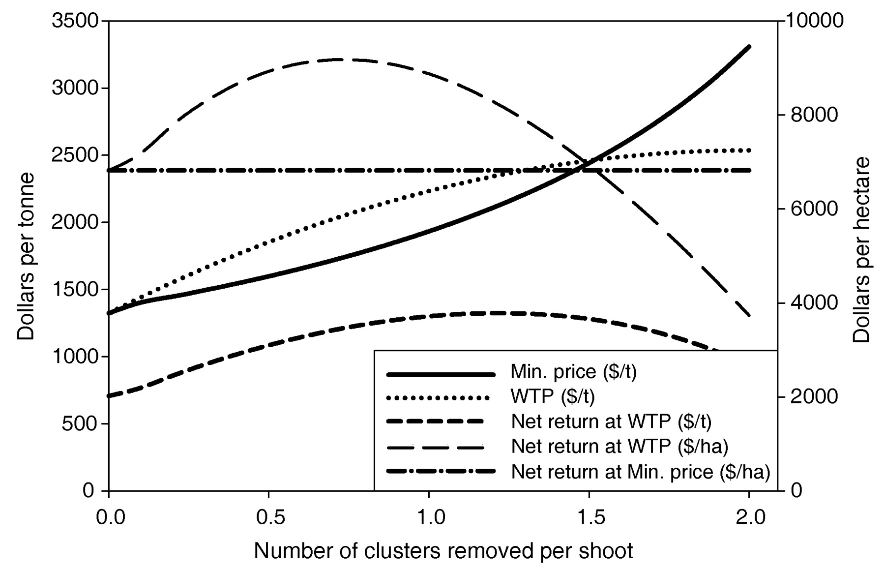
The generated WTP function is based on assumed WTP parameters of a0 = P0 = 1,323, a1 = 1,213, and a2 = -303 (the equivalent U.S. units are 1,200, 1100, and -275, respectively) (Figure 2⇓). These parameters were assigned such that for lower levels of CT, WTP prices are above the minimum price requirements (i.e., adoption of CT is economically feasible), but for higher levels of CT, WTP prices are below the minimum price requirements (i.e., CT is not economically feasible). Since the WTP prices are assumed to increase, but at a decreasing rate, this implies that as the level of CT increases, the marginal increases in WTP prices decrease and, at higher levels of CT, will not cover the increasing costs of CT.

Grower net returns per hectare as a function of level of CT and assumed willingness-to-pay (WTP) for grape quality effects from CT, as estimated by the crop-load economic model.
By design, the WTP price is maximized at x = 2 clusters removed per shoot (see equation 9), and this level of CT is not affected by grower cost or yield effects of CT. Similarly, net returns per tonne are maximized at x = 1.2 clusters removed (Figure 2⇑), where the additional production costs of CT are considered, but yield effects are not. The maximum WTP price was set to describe the WTP linkages back to the grower level. Indeed, no existing research or literature has estimated this relationship, either directly or indirectly.
After considering the assumed WTP function, additional input parameters (Table 1⇑) were substituted into equation 13 to determine the optimal level of CT for growers. In this case, using an empirical example of a Finger Lakes Riesling vineyard results in an optimal CT level of x* = 0.73. This computation maximizes grower net returns per hectare and considers all salient aspects of CT decisions: higher grape prices from increases in grape quality, higher production costs associated with CT, and lost revenue from the thinned clusters.
Grower use of model.
The model recognizes the importance of determining optimal production practices based on specific, measurable parameters. Pricing schedules for growers competing in a market with other producers must be based on a thorough understanding of such parameters. While other market factors can also influence prices received, the model allows growers to interpret the value of their own grapes as well as changes in values when alternative production practices are considered to increase grape quality. Such information should be extremely valuable in making sound production adjustments and in communications with potential buyers, based on existing market conditions. Computation of the crop-load economic metrics can be performed using basic yield and price data readily available to any vineyard manager. An Excel spreadsheet that automates the data processing is available from the corresponding author.
Considerations for training systems and regions.
This model is designed to enhance decision-making acuity among winegrape growers who use CT to reduce crop load or advance fruit maturity. It is suitable for application to vineyard operations in warm and cool climates, for red and white grapes of any commercially grown species (e.g., Vitis vinifera, Vitis sp., Vitis labruscana), and for any canopy training system. In addition, the model can be tailored constructively in appellations where yield and cost structures vary widely among individual producers. Although the model is robust enough to reveal opportunities for greatly enhanced efficiency, its accuracy depends on the accuracy of the input parameter data used for its computations. This underscores the importance of detailed record keeping and a data-driven management philosophy in vineyard operations.
Additional applications.
The model described here not only is useful in a single-producer competitive market but also can be generalized to establish uniform pricing or optimal yields for cooperative grower organizations, as long as data for cost and yield input parameters are adjusted accordingly. The response curves generated could be used in strategic planning for vineyard operations to streamline the annual budget planning process across functional areas of the vineyard, winery, and sales operation. Other vineyard management aspects that could be improved by these production optimality metrics include disease and pest pressure control, non-CT canopy-management practices, and calibration of equipment usage versus hand-labor requirements.
Directions for future research.
This model can be expanded further to include and interpret delayed effects on fruit quality valuations and vine health, which may span numerous more complicated physiological factors over time, as the long-term effects of CT practices become apparent. Additionally, optimal crop-load management practices could be defined in context with wine quality and consumer response to wines made from grapes at different crop-load levels. It would be instructive to evaluate changes in crop-load indices, long-term vine health, and links between grape and wine prices based on changes in both grape and wine-quality parameters, including those related to wine flavor chemistry. Long-term data collection through viticultural field research, winemaking, flavor chemistry analysis, and consumer WTP response surveys would be necessary to enhance the model’s specificity toward particular wine styles. The development of a more complex utility-theoretic behavioral choice framework based on specific wine styles could equally serve grower, winery, and consumer objectives for quality improvement and economic sustainability.
Conclusion
New analytical methods use commonly available vineyard data for yields and costs to reveal previously overlooked viticultural and economic efficiencies. When applied to sample data, this tailored economic model demonstrated that growers can determine their required price at a given yield, and their optimal yield at a given WTP price. These metrics allow growers to take a more active role in the competitive environment of grape contract pricing and make specific, quantitatively justified CT decisions in the field. The ultimate goal of establishing such a model is to enhance the decision-making acuity of growers with respect to grapevine crop-load management, while simultaneously strengthening the economic sustainability of vineyard operations. It would be helpful if publications relating to CT provide as much detail as possible about production costs, yields, prices, and grape quality parameters so that this model can be applied to the data and economic comparisons can be made between different crop-load levels.
Footnotes
Acknowledgments: This manuscript is based upon work supported by the New York Wine and Grape Foundation.
The authors thank Professor emeritus Gerald B. White for his helpful review of the manuscript. A spreadsheet with all necessary calculations to use the model described in this article is available from the corresponding author.
- Received April 2009.
- Revision received July 2009.
- Accepted August 2009.
- Published online March 2010
- Copyright © 2010 by the American Society for Enology and Viticulture
Literature Cited
Vol 61 Issue 1


Jump to section
Related Articles
Cited By...
More from this TOC section
Similar Articles